Mooney-Rivlin Model
When solid materials are subjected to a load, they undergo elastic deformations and when the load is removed, they return to their original dimensions within the range where the relationship between load and strain is linear, which is typically very narrow. Rubber-like materials, on the other hand, show elastic behavior over a much wider range of deformations (in some cases up to 1000%). However, these so called hyperelastic materials typically show a nonlinear elastic relationship between load and strain.
The elastic behavior of rubbery materials can be derived from the strain energy density function. A model based on this function was developed by Melvin Mooney in 1940 and expressed in terms of invariants by Ronald Rivlin in 1948.1,2 In his model, the strain energy density function is assumed to be a linear combination of three invariants of the Cauchy strain tensor. This tensor is symmetric by definition and can be converted into a diagonal form by a suitable rotation of the coordinate system. Then the Cauchy strain tensor C includes only the reciprocal extension or stretch ratios, defined as the deformations of a cubic volume element along the principal axes, λi = dLi / dLi,0:
![]()
Alternatively, the strain energy density function can be expressed by the Finger strain tensor B which is defined as the reciprocal of the Cauchy deformation tensor B = C-1. The diagonal form of this tensor is given by3
![]()
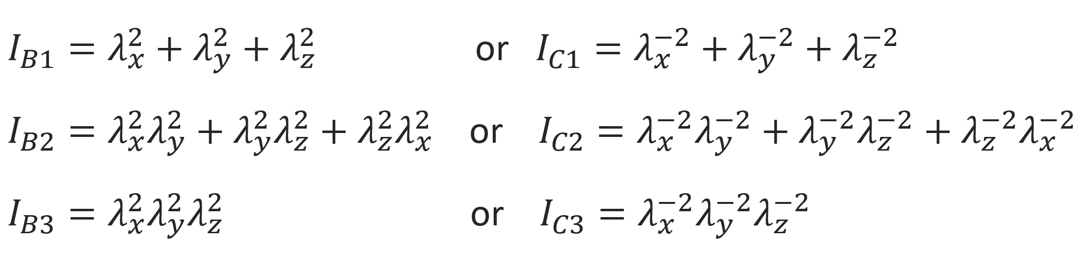
The strain tensor possesses three invariants which can be expressed in terms of the Cauchy or Finger tensor components:4-7
The elastic behavior of hyperelastic materials, i.e., their stress-strain relationships can be derived from the strain energy density w, which is assumed to be solely a function of these three strain invariants:
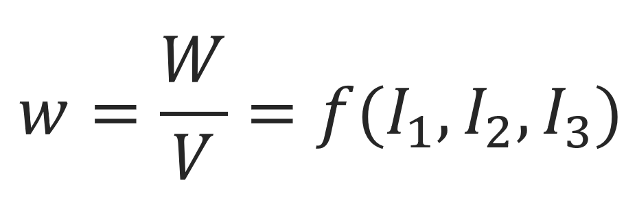
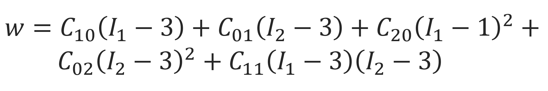
This function is the energy stored in the elastomer per initial cubic unit volume. It can be written as a power series of differences of the three invariants from their values in the undeformed state (λx = λy = λz = 1):
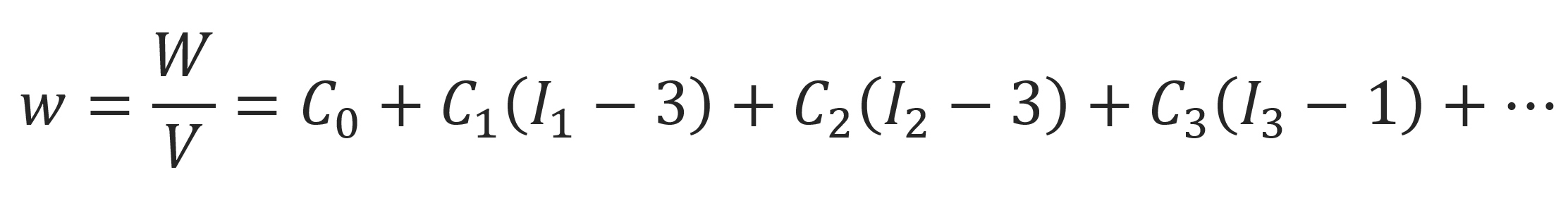
where the Ci's are empirically model constants that can be determined by fitting the stress-strain data to the model. Note, the second term in this series is identical with the strain energy density calculated with the classical fixed junction model:
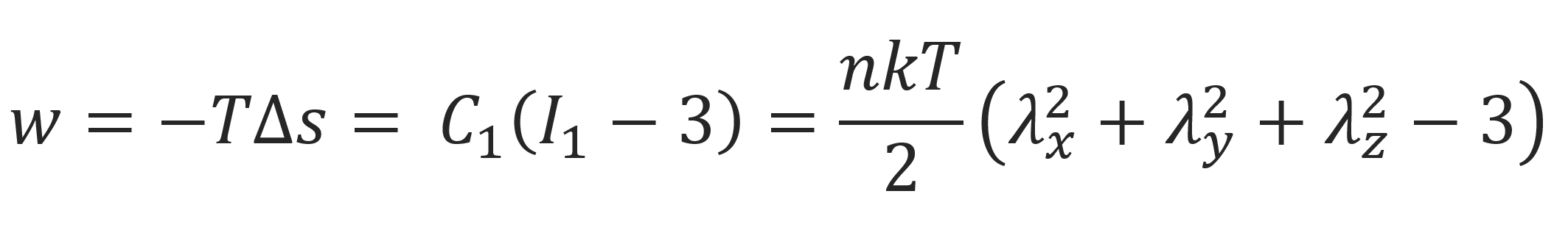
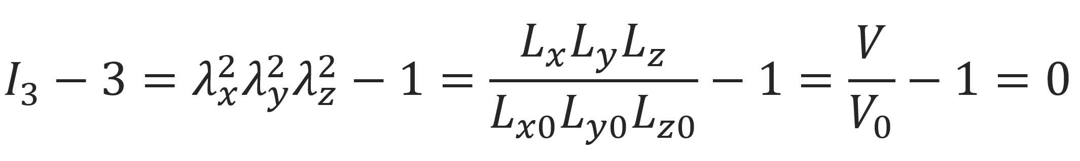
The third term describes the deviation from the neo-Hookean model. The fourth term is zero, if the material is an incompressible polymer network:
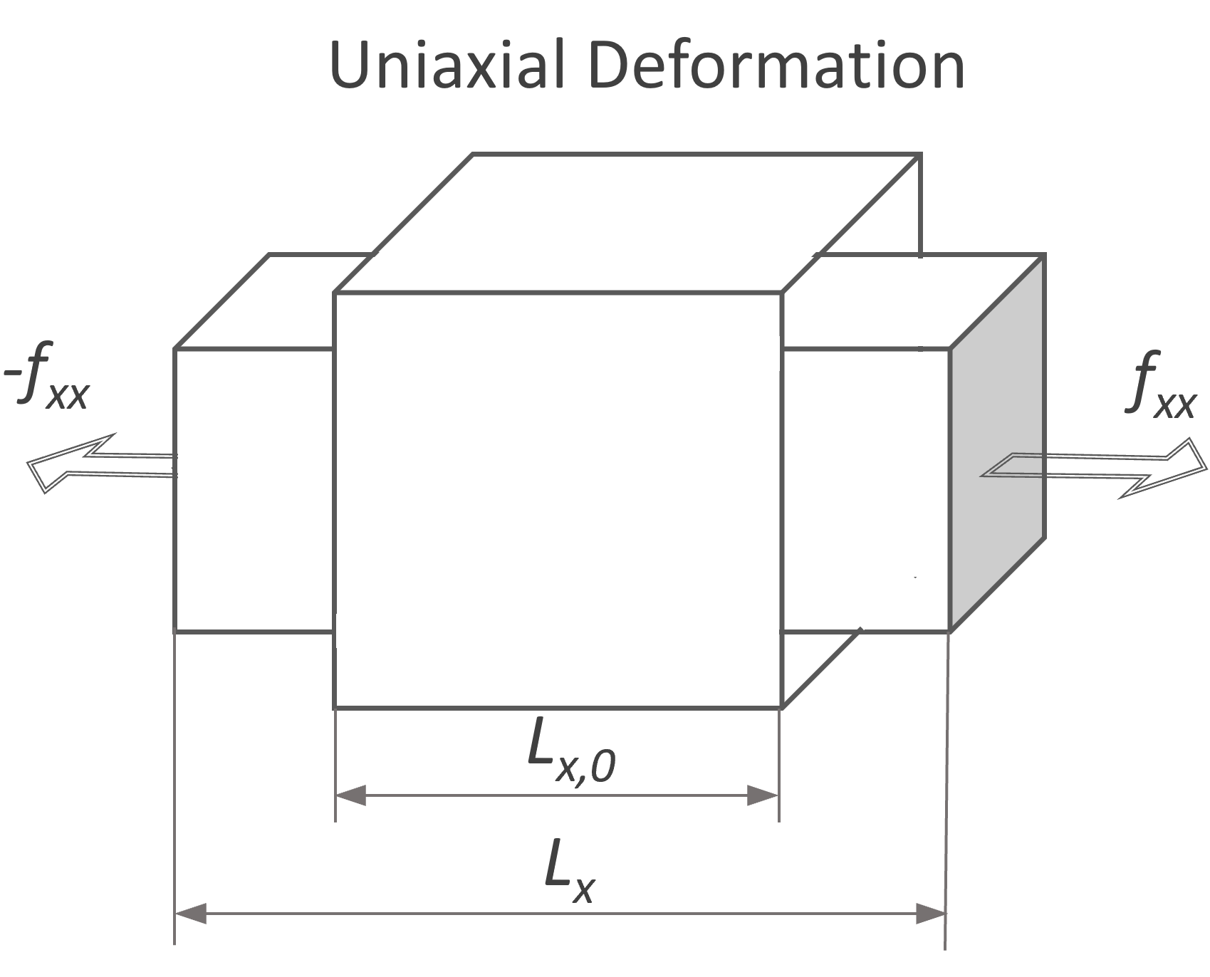
Example: Uniaxial deformation of incompressible materials:
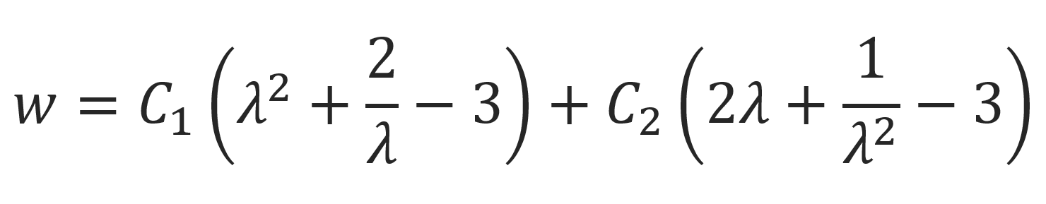
A popular model of an incompressible Mooney-Rivlin material is based on a combination of the linear terms of the power series of the deformation energy density:8,9
![]()
For unilateral deformation: λx = λ; λy = λz = λ-1/2 (see table below), the Mooney-Rivlin equation reads in terms of the extension ratios
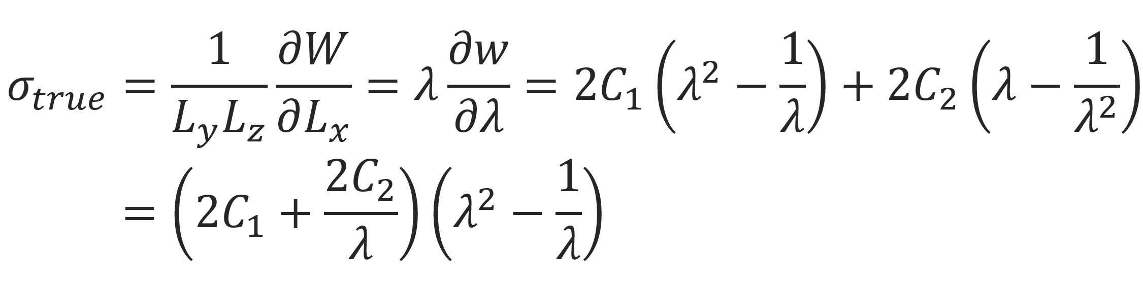
The true stress can be obtained by performing the differentiation with respect to the extension:
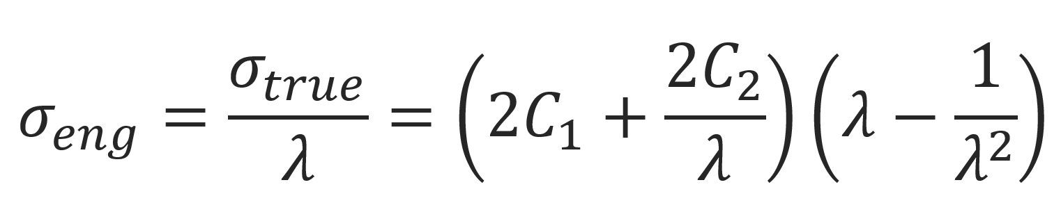
The engineering stress can be obtained by dividing the true strain by the extension ratio:
For 2C1 = G and C2 = 0, the Mooney-Rivlin model is identical with the neo-Hookean model.
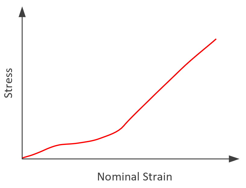
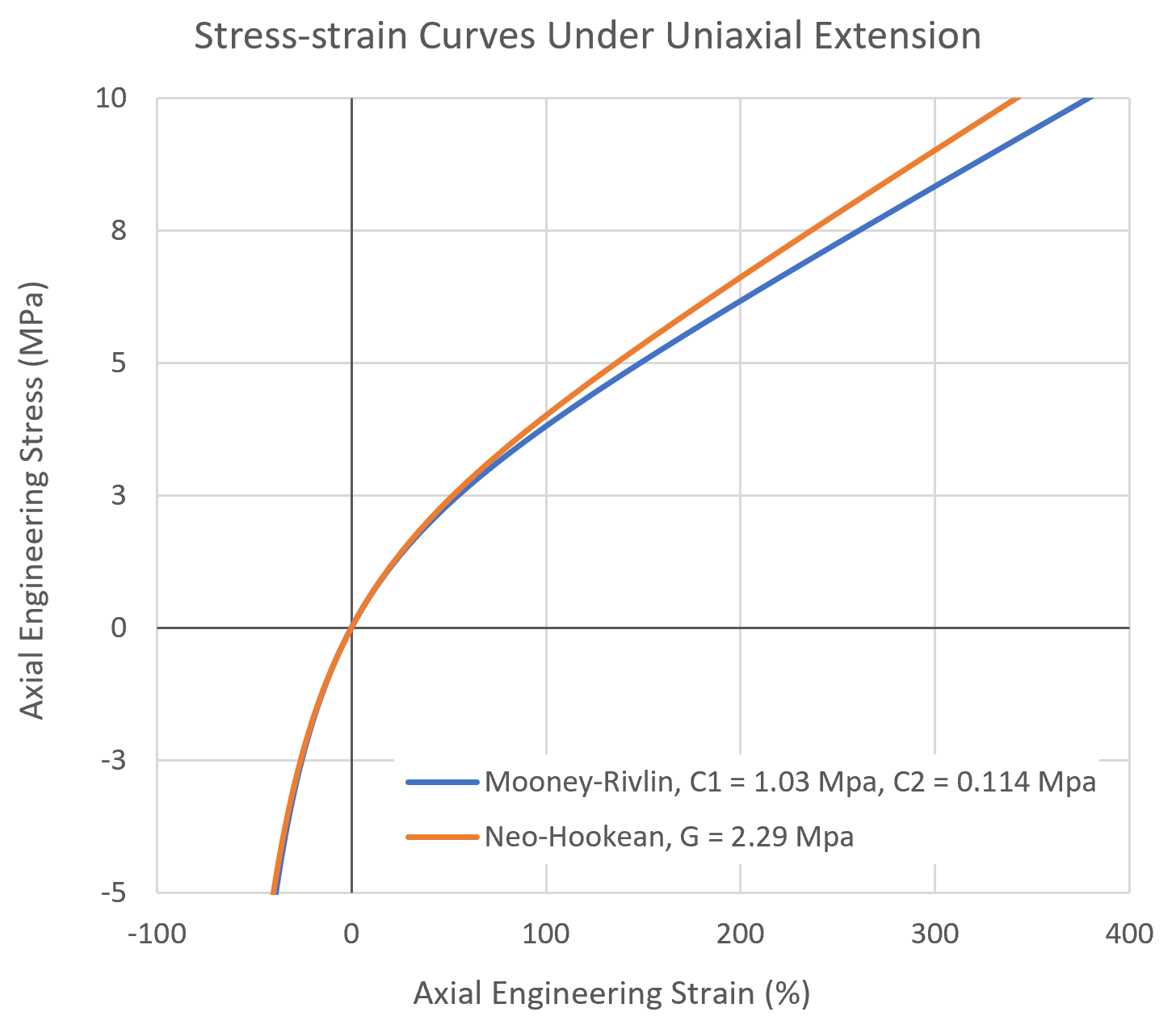
The figure below shows the stress-strain curves under uniaxial extension for the Neo-Hookean model and the 2-parameter Mooney-Rivlin model.
For small extensions, both models provide similar stress-strain curves, whereas for strain values above 50 percent the Mooney-Rivlin model noticeably deviates from the fixed junction model.
The two and three constant Mooney-Rivlin models have some major limitations when predicting the behavior of elastomers at large deformations. To obtain more accurate results in rubber-like materials, more terms of the power series have to be included. Often a five parameter Mooney-Rivlin model is chosen:
As has been shown by Rao et al., the five and nine parameter Mooney-Rivlin models give curve fits that reasonably reproduce the mechanical behavior at large strains.9 If this apporach does not give the desired accuracy, more advanced hyperelastic models have to be employed.10
| Strain Modes | Strain Relations | |
3-Dimensional Strain (Pressure) |
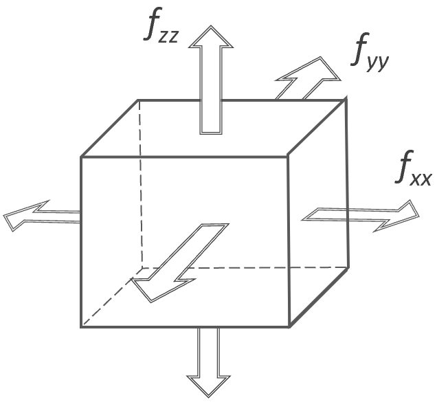 |
λxλyλz = 1 (ΔV = 0) |
Unilateral Strain in |
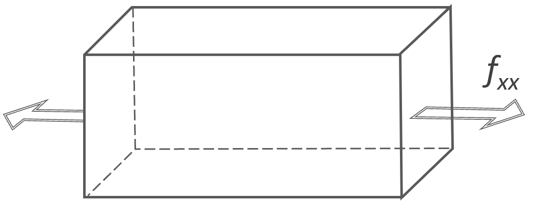 |
λx = λ; λy = λz = λ-1/2 |
2-Dimensional Strain in |
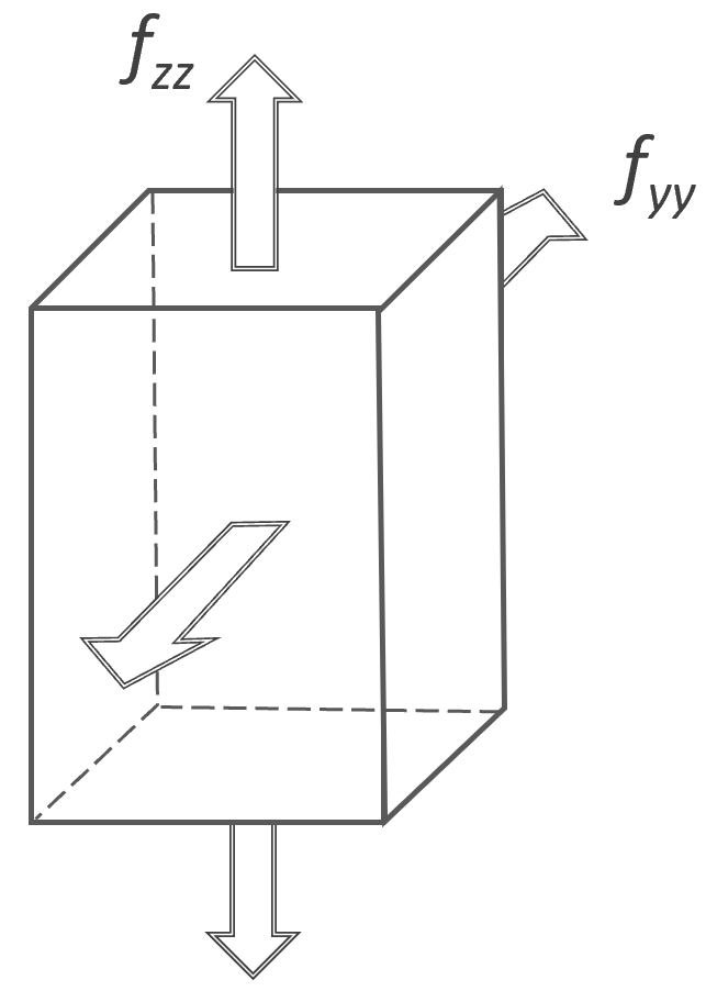 |
λy = λz = λ; λx = λ-2 |
Pure Shear Strain |
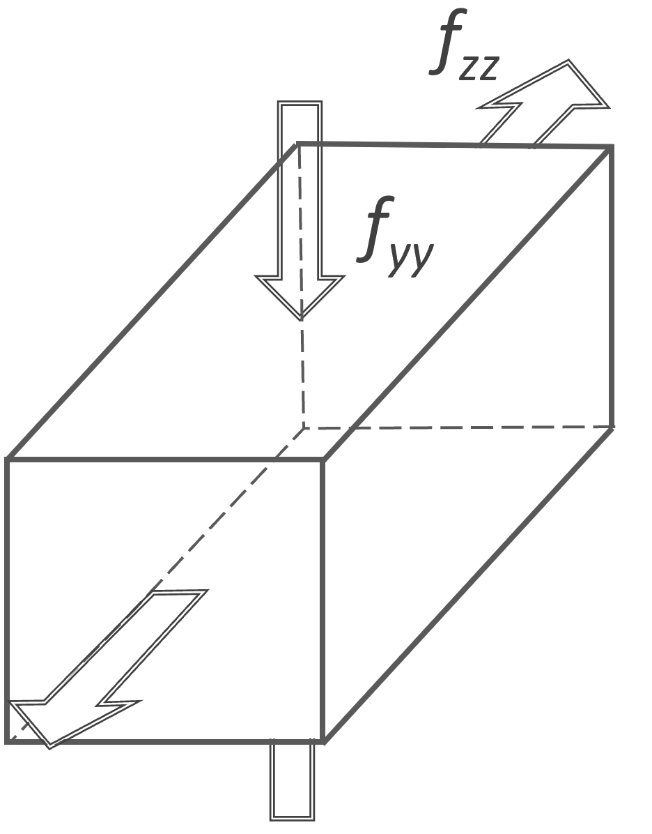 |
λx = λ; λy = 1; λz = λ-1 |
Simple Shear Strain |
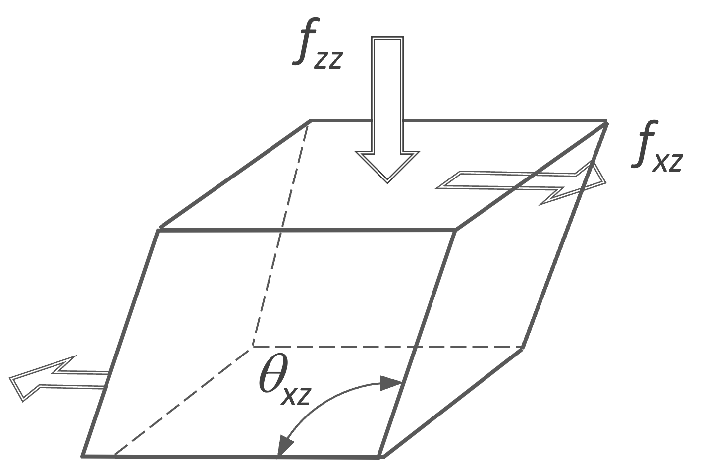 |
γ = tan (θxz - π/2); |
References & Further Reading
- R.S. Rivlin, Math. & Phys. Sci., Vol. 240 A, 491-508 (1948)
- M. Mooney, J. Appl. Phys., Vol 11, 582-592 (1940)
- The Finger tensor, also known as the Cauchy-Green or Green strain tensor, is a symmetric tensor that has real positive eigenvalues. Its values are squares of stretch ratios defined as the ratio of the length of a stretched line element to the length of the corresponding undeformed line element: λ2 = (|dL| / |dL0|)2.
- G. Strobl, The Physics of Polymers, 3rd Edition, Heidelberg 2007
- M. Rubinstein and R. Colby, Polymer Physics, 1st Ed., Oxford University Press (2003)
- L.R.G. Treloar, The Physics of Rubber Elasticity, Oxford 1949
- They are called invariants because they do not change when the coordinate system is transformed (rotated).
- B. Kim, S.B. Lee, J. Lee, S. Chom H. Parlm S. Yeom and S.H. Park, Int. J. Precis. Eng. Manuf., Vol. 13, No. 5, pp. 759-764 (2012)
- M. Ramamohan Rao and M.R.S. Satayanarayana, Int. J. Eng. Res. & Tech., Vol. 7 (3) (2019)
- R. Tobajas, E. Ibarz and L. Gracia, Proc. of the 2nd Intl. Electr. Conf. on Mat., MDPI (2016)